What role does the campaign play in determining election outcomes?
Presidential campaigns have three main purposes — to convince donors, persuade voters, and mobilize the electorate. Last weeks blog discussed one of the mechanisms by which campaigns seek to attain this goal: the air war of mass media campaign advertising. This week’s post will explore the ground game, through which campaigns attempt to target individual voters.
Individual targeting, which often takes the form of phone calls, door-knocks, and text messages out of localized field offices, attempts to psychologically target a voter for the sake of persuasion and mobilization. Indeed, the ground game used to be the only way for campaigns to get out the vote and spread their message. In an age of mass media, however, the air war became increasingly popular as a way of marketing candidates to a large audience like products. The turning point occurred in the Obama McCain race, when then Senator Obama, aware of the over-saturation of campaign advertising and hoping to connect directly with emerging sectors of the electorate, decided to re-focus on the ground game.
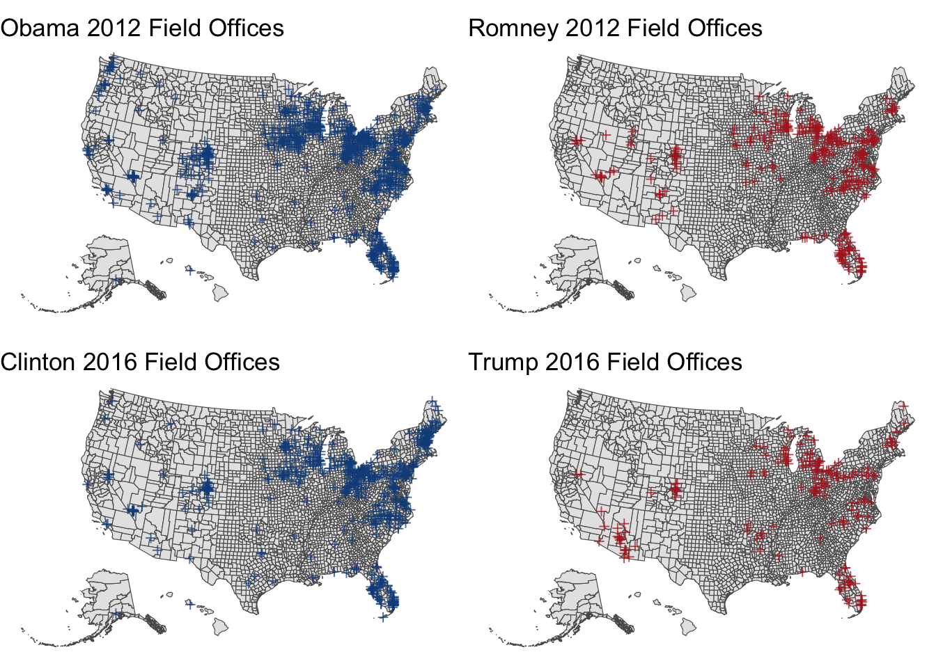
The first graphic shows the difference in field office location between the 2012 Obama v. Romney campaign and the 2016 Clinton v. Trump campaign. This graphic not only displays the different numbers of field offices between candidates and years — In 2012 Obama ran 965 field offices while Romney had 283, in 2016 Clinton had 538 to Trump’s 165 — but also the various locations of said offices.
##
|
| | 0%
|
| | 1%
|
|= | 1%
|
|= | 2%
|
|== | 2%
|
|== | 3%
|
|=== | 4%
|
|=== | 5%
|
|==== | 5%
|
|==== | 6%
|
|===== | 6%
|
|===== | 7%
|
|===== | 8%
|
|====== | 8%
|
|====== | 9%
|
|======= | 9%
|
|======= | 10%
|
|======== | 11%
|
|======== | 12%
|
|========= | 12%
|
|========= | 13%
|
|========== | 14%
|
|========== | 15%
|
|=========== | 15%
|
|=========== | 16%
|
|============ | 17%
|
|============ | 18%
|
|============= | 18%
|
|============= | 19%
|
|============== | 20%
|
|============== | 21%
|
|=============== | 21%
|
|=============== | 22%
|
|================ | 23%
|
|================= | 24%
|
|================= | 25%
|
|================== | 25%
|
|================== | 26%
|
|=================== | 26%
|
|=================== | 27%
|
|=================== | 28%
|
|==================== | 28%
|
|==================== | 29%
|
|===================== | 29%
|
|===================== | 30%
|
|===================== | 31%
|
|====================== | 31%
|
|====================== | 32%
|
|======================= | 32%
|
|======================= | 33%
|
|======================== | 34%
|
|======================== | 35%
|
|========================= | 35%
|
|========================= | 36%
|
|========================== | 36%
|
|========================== | 37%
|
|========================== | 38%
|
|=========================== | 38%
|
|=========================== | 39%
|
|============================ | 40%
|
|============================= | 41%
|
|============================= | 42%
|
|============================== | 42%
|
|============================== | 43%
|
|=============================== | 44%
|
|=============================== | 45%
|
|================================ | 45%
|
|================================ | 46%
|
|================================= | 46%
|
|================================= | 47%
|
|================================= | 48%
|
|================================== | 48%
|
|================================== | 49%
|
|=================================== | 49%
|
|=================================== | 50%
|
|=================================== | 51%
|
|==================================== | 51%
|
|==================================== | 52%
|
|===================================== | 52%
|
|===================================== | 53%
|
|===================================== | 54%
|
|====================================== | 54%
|
|====================================== | 55%
|
|======================================= | 55%
|
|======================================= | 56%
|
|======================================== | 57%
|
|======================================== | 58%
|
|========================================= | 58%
|
|========================================= | 59%
|
|========================================== | 59%
|
|========================================== | 60%
|
|========================================== | 61%
|
|=========================================== | 61%
|
|=========================================== | 62%
|
|============================================ | 62%
|
|============================================ | 63%
|
|============================================= | 64%
|
|============================================= | 65%
|
|============================================== | 65%
|
|============================================== | 66%
|
|=============================================== | 66%
|
|=============================================== | 67%
|
|=============================================== | 68%
|
|================================================ | 68%
|
|================================================ | 69%
|
|================================================= | 69%
|
|================================================= | 70%
|
|================================================= | 71%
|
|================================================== | 71%
|
|================================================== | 72%
|
|==================================================== | 75%
|
|===================================================== | 75%
|
|===================================================== | 76%
|
|====================================================== | 77%
|
|====================================================== | 78%
|
|======================================================= | 78%
|
|======================================================= | 79%
|
|======================================================== | 79%
|
|======================================================== | 80%
|
|======================================================== | 81%
|
|========================================================= | 81%
|
|========================================================== | 82%
|
|========================================================== | 83%
|
|=========================================================== | 84%
|
|============================================================ | 85%
|
|============================================================ | 86%
|
|============================================================= | 87%
|
|============================================================== | 88%
|
|============================================================== | 89%
|
|=============================================================== | 89%
|
|=============================================================== | 90%
|
|================================================================ | 91%
|
|================================================================ | 92%
|
|================================================================= | 92%
|
|================================================================= | 93%
|
|================================================================== | 94%
|
|================================================================== | 95%
|
|=================================================================== | 95%
|
|======================================================================| 100%
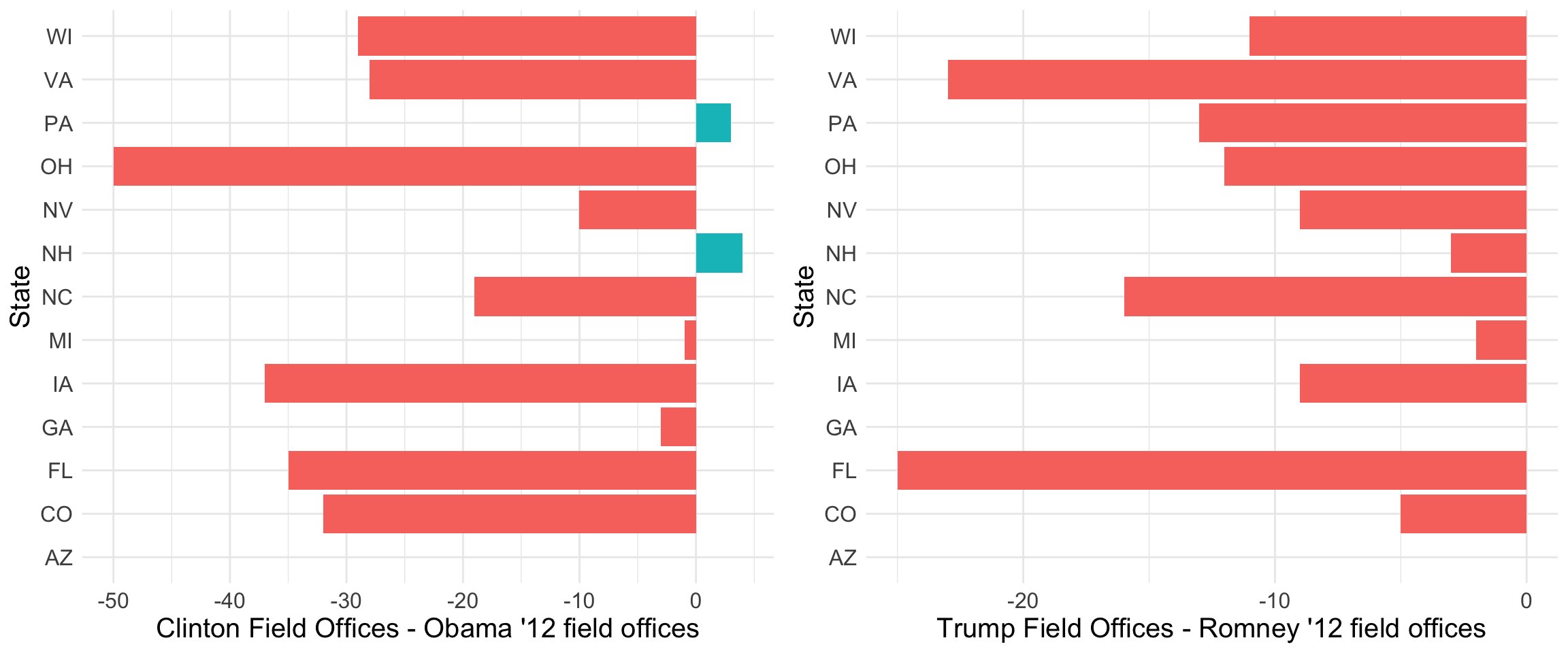
The second graphic displays the difference in field offices between Clinton in 2016 and Obama in 2012 as well as Trump in 2016 and Romney in 2012. As expressed in the graph, Clinton utilized significantly less field offices than Obama, only adding in Pennsylvania — 54 to 57 offices — and New Hampshire — 22 to 26 offices. The more drastic shift, however, is seen from Romney to Trump, wherein the number of field offices decreases across all states.
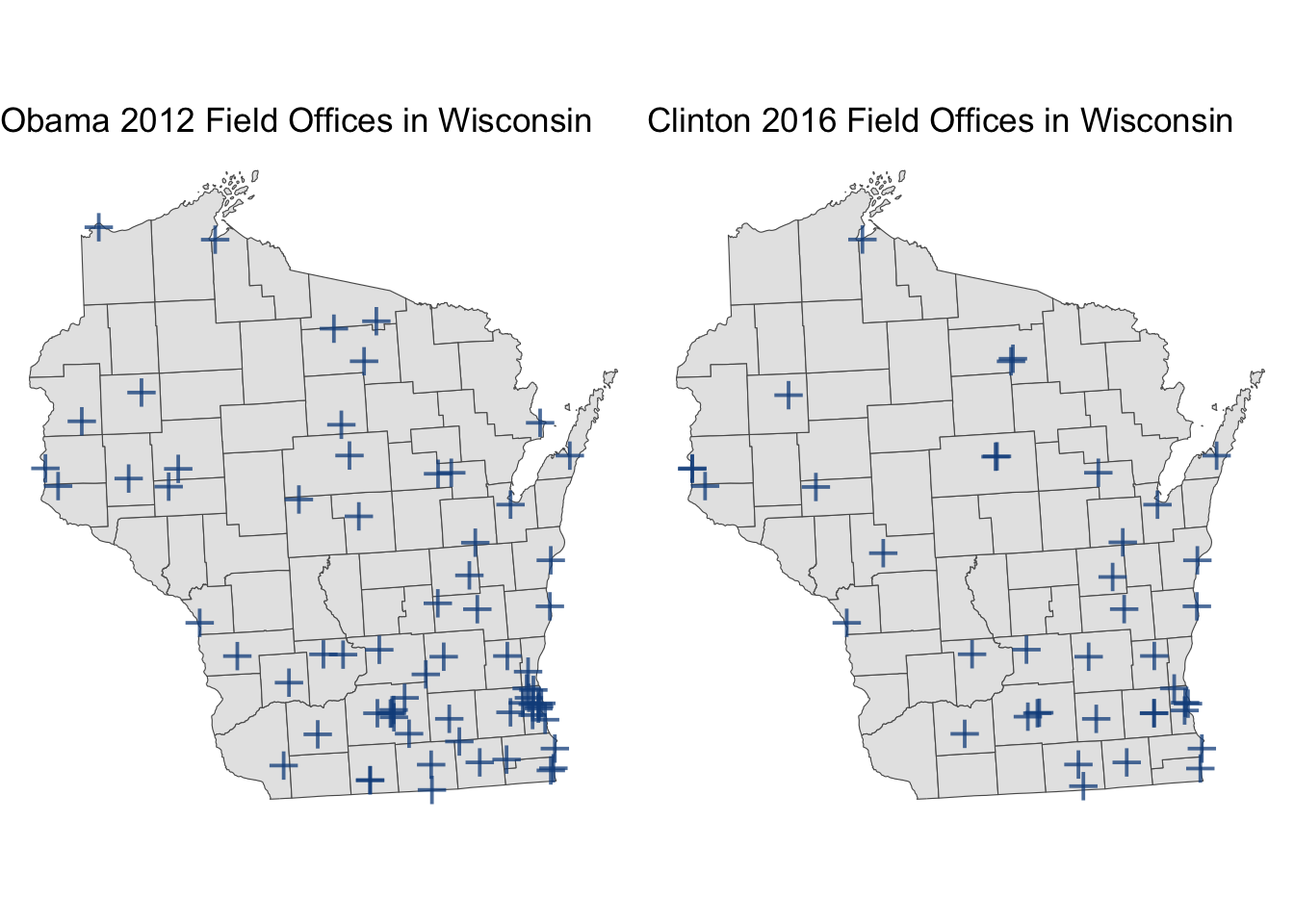
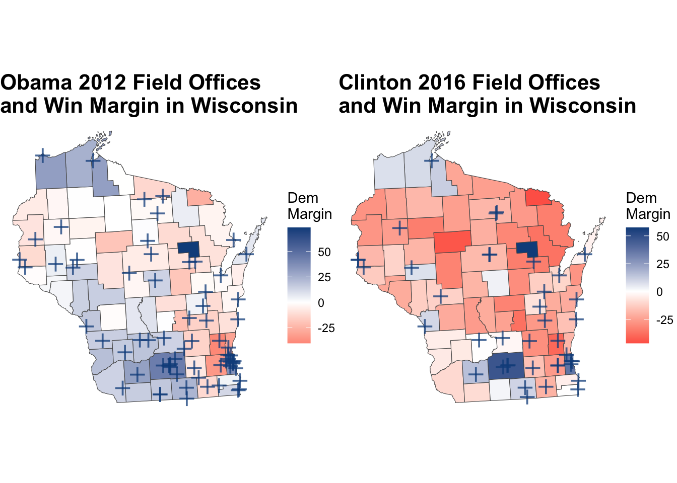
When it comes to the efficacy of field offices, one of the most popular narratives surrounding the shift in campaign strategy from Obama to Clinton that is visualized above asserts that Clinton’s removal of Wisconsin field offices lost her the state in 2016. Below, this effect is visualized, displaying that some areas where Clinton decreased the number of field offices from 2012 to 2016 appeared to swing Republican.
Does the ground game truly influence voters?
Though the analysis above is interesting, it fails to conclusively display any relationship between the ground game and voting behavior. Since campaigns are measured by their ability to both persuade and mobilize voters, these relationship between the ground game and these two effects will be explored below.
The existing political science literature asserts that the ability of the ground game to persuade voters is negligible. Indeed, in an aggregate study of 49 field experiments, scholars Kalla and Brockman found that persuasion efforts of ground campaigns are almost entirely ineffective (Kalla and Brockman, 2018). The mobilization effect, however, is found to be incredibly significant. Indeed, in an experiment which compared battleground states (where there is a ground game) and non-swing states (without one) in areas where there is a spillover media market, ensuring that the air war remains constant, Enos and Fowler found that the ground game led to an increase in turnout around 6% (Enos and Fowler, 2016).
The regressions below first outlines where campaigns choose to build field offices as well as the efficacy of said offices on turnout and vote share. According to the first model, field office placement is most related to whether or not the state is a battle ground state, the size of the state’s population, and the presence of the other campaign’s field offices. All three variables are statistically significant at the 0.001 level.
##
## Call:
## lm(formula = romney12fo ~ obama12fo + swing + core_dem + swing:obama12fo +
##     core_dem:obama12fo + battle + medage08 + pop2008 + pop2008^2 +
##     medinc08 + black + hispanic + pc_less_hs00 + pc_degree00 +
##     as.factor(state), data = fo_2012)
##
## Residuals:
##      Min       1Q   Median       3Q      Max
## -1.55064 -0.04172  0.00610  0.03253  2.89802
##
## Coefficients: (1 not defined because of singularities)
##                                  Estimate Std. Error t value Pr(>|t|)
## (Intercept)                     1.171e-03  7.927e-02   0.015 0.988214
## obama12fo                       3.740e-01  1.969e-02  18.997  < 2e-16 ***
## swingTRUE                      -1.173e-02  1.104e-02  -1.062 0.288307
## core_demTRUE                    3.699e-03  2.658e-02   0.139 0.889316
## battleTRUE                      1.416e-02  4.187e-02   0.338 0.735359
## medage08                       -8.876e-04  1.096e-03  -0.810 0.418072
## pop2008                        -6.555e-08  1.623e-08  -4.040 5.49e-05 ***
## medinc08                        9.971e-07  6.304e-07   1.582 0.113806
## black                           5.015e-05  4.558e-04   0.110 0.912389
## hispanic                        7.894e-04  5.666e-04   1.393 0.163670
## pc_less_hs00                   -1.296e-01  1.119e-01  -1.158 0.246867
## pc_degree00                     3.053e-01  9.661e-02   3.160 0.001593 **
## as.factor(state)Arizona        -5.011e-02  6.749e-02  -0.743 0.457808
## as.factor(state)Arkansas        1.264e-03  3.903e-02   0.032 0.974170
## as.factor(state)California     -9.946e-02  4.476e-02  -2.222 0.026359 *
## as.factor(state)Colorado       -1.729e-01  4.072e-02  -4.246 2.24e-05 ***
## as.factor(state)Connecticut    -1.446e-01  8.620e-02  -1.677 0.093559 .
## as.factor(state)Delaware       -1.349e-01  1.337e-01  -1.009 0.312995
## as.factor(state)Florida         2.438e-01  3.935e-02   6.194 6.63e-10 ***
## as.factor(state)Georgia        -1.834e-02  3.307e-02  -0.554 0.579361
## as.factor(state)Hawaii         -1.261e-01  1.175e-01  -1.074 0.282984
## as.factor(state)Idaho          -5.436e-02  4.705e-02  -1.156 0.247975
## as.factor(state)Illinois       -3.319e-02  3.792e-02  -0.875 0.381441
## as.factor(state)Indiana        -3.192e-02  3.899e-02  -0.819 0.413025
## as.factor(state)Iowa           -1.147e-01  3.510e-02  -3.266 0.001101 **
## as.factor(state)Kansas         -4.617e-02  3.913e-02  -1.180 0.238158
## as.factor(state)Kentucky        8.010e-03  3.627e-02   0.221 0.825214
## as.factor(state)Louisiana      -9.488e-04  3.961e-02  -0.024 0.980893
## as.factor(state)Maine          -8.801e-02  6.498e-02  -1.354 0.175730
## as.factor(state)Maryland       -7.396e-02  5.526e-02  -1.338 0.180852
## as.factor(state)Massachusetts  -1.097e-01  7.028e-02  -1.561 0.118545
## as.factor(state)Michigan        1.746e-01  4.006e-02   4.357 1.36e-05 ***
## as.factor(state)Minnesota      -7.317e-02  3.997e-02  -1.831 0.067252 .
## as.factor(state)Mississippi     2.023e-04  3.776e-02   0.005 0.995726
## as.factor(state)Missouri        5.894e-02  3.679e-02   1.602 0.109268
## as.factor(state)Montana        -4.981e-02  4.458e-02  -1.117 0.263959
## as.factor(state)Nebraska       -3.104e-02  4.091e-02  -0.759 0.448090
## as.factor(state)Nevada          2.077e-01  6.176e-02   3.362 0.000783 ***
## as.factor(state)New Hampshire   1.776e-01  7.679e-02   2.313 0.020769 *
## as.factor(state)New Jersey     -8.703e-02  5.920e-02  -1.470 0.141612
## as.factor(state)New Mexico      7.959e-02  5.523e-02   1.441 0.149674
## as.factor(state)New York       -5.593e-02  4.191e-02  -1.334 0.182146
## as.factor(state)North Carolina  5.353e-02  3.616e-02   1.481 0.138812
## as.factor(state)North Dakota   -3.171e-02  4.403e-02  -0.720 0.471518
## as.factor(state)Ohio           -3.137e-02  3.631e-02  -0.864 0.387668
## as.factor(state)Oklahoma       -2.190e-02  3.969e-02  -0.552 0.581226
## as.factor(state)Oregon         -9.337e-02  4.951e-02  -1.886 0.059431 .
## as.factor(state)Pennsylvania    1.112e-01  3.873e-02   2.870 0.004134 **
## as.factor(state)Rhode Island   -1.231e-01  1.062e-01  -1.159 0.246358
## as.factor(state)South Carolina -2.669e-02  4.351e-02  -0.613 0.539614
## as.factor(state)South Dakota   -3.257e-02  4.182e-02  -0.779 0.436188
## as.factor(state)Tennessee       5.134e-03  3.758e-02   0.137 0.891342
## as.factor(state)Texas          -3.726e-02  3.539e-02  -1.053 0.292533
## as.factor(state)Utah            5.975e-02  5.375e-02   1.112 0.266375
## as.factor(state)Vermont        -7.979e-02  6.821e-02  -1.170 0.242144
## as.factor(state)Virginia        2.658e-02  3.613e-02   0.736 0.461878
## as.factor(state)Washington     -1.220e-01  4.823e-02  -2.529 0.011486 *
## as.factor(state)West Virginia   2.856e-03  4.291e-02   0.067 0.946938
## as.factor(state)Wisconsin              NA         NA      NA       NA
## as.factor(state)Wyoming        -6.440e-02  5.833e-02  -1.104 0.269585
## obama12fo:swingTRUE            -8.084e-02  1.962e-02  -4.121 3.88e-05 ***
## obama12fo:core_demTRUE         -1.643e-01  2.349e-02  -6.998 3.18e-12 ***
## ---
## Signif. codes:  0 '***' 0.001 '**' 0.01 '*' 0.05 '.' 0.1 ' ' 1
##
## Residual standard error: 0.2258 on 3049 degrees of freedom
##   (3 observations deleted due to missingness)
## Multiple R-squared:  0.6507,	Adjusted R-squared:  0.6439
## F-statistic: 94.68 on 60 and 3049 DF,  p-value: < 2.2e-16
| Variable | Obama 2012 Estimate | Obama 2012 Std. Error | Romney 2012 Estimate | Romney 2012 Std. Error |
|---|---|---|---|---|
| (Intercept) | -0.340 | 0.196 | 0.001 | 0.079 |
| romney12fo | 2.546 | 0.114 | NA | NA |
| swingTRUE | 0.001 | 0.055 | -0.012 | 0.011 |
| core_repTRUE | 0.007 | 0.061 | NA | NA |
| battleTRUE | 0.541 | 0.096 | 0.014 | 0.042 |
| medage08 | 0.000 | 0.003 | -0.001 | 0.001 |
| pop2008 | 0.000 | 0.000 | 0.000 | 0.000 |
| medinc08 | 0.000 | 0.000 | 0.000 | 0.000 |
| black | 0.003 | 0.001 | 0.000 | 0.000 |
| hispanic | 0.000 | 0.001 | 0.001 | 0.001 |
| pc_less_hs00 | 0.506 | 0.259 | -0.130 | 0.112 |
| pc_degree00 | 0.951 | 0.223 | 0.305 | 0.097 |
| as.factor(state)Arizona | -0.028 | 0.156 | -0.050 | 0.067 |
| as.factor(state)Arkansas | 0.076 | 0.090 | 0.001 | 0.039 |
| as.factor(state)California | -0.076 | 0.104 | -0.099 | 0.045 |
| as.factor(state)Colorado | 0.163 | 0.094 | -0.173 | 0.041 |
| as.factor(state)Connecticut | 0.036 | 0.200 | -0.145 | 0.086 |
| as.factor(state)Delaware | 0.207 | 0.309 | -0.135 | 0.134 |
| as.factor(state)Florida | -0.290 | 0.091 | 0.244 | 0.039 |
| as.factor(state)Georgia | 0.029 | 0.077 | -0.018 | 0.033 |
| as.factor(state)Hawaii | 0.179 | 0.272 | -0.126 | 0.117 |
| as.factor(state)Idaho | 0.154 | 0.109 | -0.054 | 0.047 |
| as.factor(state)Illinois | 0.117 | 0.088 | -0.033 | 0.038 |
| as.factor(state)Indiana | 0.140 | 0.090 | -0.032 | 0.039 |
| as.factor(state)Iowa | 0.081 | 0.081 | -0.115 | 0.035 |
| as.factor(state)Kansas | 0.147 | 0.091 | -0.046 | 0.039 |
| as.factor(state)Kentucky | 0.105 | 0.084 | 0.008 | 0.036 |
| as.factor(state)Louisiana | -0.004 | 0.092 | -0.001 | 0.040 |
| as.factor(state)Maine | 0.274 | 0.150 | -0.088 | 0.065 |
| as.factor(state)Maryland | -0.047 | 0.128 | -0.074 | 0.055 |
| as.factor(state)Massachusetts | -0.118 | 0.163 | -0.110 | 0.070 |
| as.factor(state)Michigan | -0.083 | 0.093 | 0.175 | 0.040 |
| as.factor(state)Minnesota | 0.271 | 0.092 | -0.073 | 0.040 |
| as.factor(state)Mississippi | -0.034 | 0.087 | 0.000 | 0.038 |
| as.factor(state)Missouri | 0.040 | 0.085 | 0.059 | 0.037 |
| as.factor(state)Montana | 0.167 | 0.103 | -0.050 | 0.045 |
| as.factor(state)Nebraska | 0.167 | 0.095 | -0.031 | 0.041 |
| as.factor(state)Nevada | -0.054 | 0.143 | 0.208 | 0.062 |
| as.factor(state)New Hampshire | 0.091 | 0.178 | 0.178 | 0.077 |
| as.factor(state)New Jersey | -0.166 | 0.137 | -0.087 | 0.059 |
| as.factor(state)New Mexico | 0.093 | 0.128 | 0.080 | 0.055 |
| as.factor(state)New York | -0.019 | 0.097 | -0.056 | 0.042 |
| as.factor(state)North Carolina | 0.230 | 0.084 | 0.054 | 0.036 |
| as.factor(state)North Dakota | 0.163 | 0.102 | -0.032 | 0.044 |
| as.factor(state)Ohio | 0.305 | 0.084 | -0.031 | 0.036 |
| as.factor(state)Oklahoma | 0.113 | 0.092 | -0.022 | 0.040 |
| as.factor(state)Oregon | 0.270 | 0.115 | -0.093 | 0.050 |
| as.factor(state)Pennsylvania | -0.351 | 0.089 | 0.111 | 0.039 |
| as.factor(state)Rhode Island | 0.117 | 0.246 | -0.123 | 0.106 |
| as.factor(state)South Carolina | -0.003 | 0.101 | -0.027 | 0.044 |
| as.factor(state)South Dakota | 0.156 | 0.097 | -0.033 | 0.042 |
| as.factor(state)Tennessee | 0.081 | 0.087 | 0.005 | 0.038 |
| as.factor(state)Texas | 0.044 | 0.082 | -0.037 | 0.035 |
| as.factor(state)Utah | 0.036 | 0.124 | 0.060 | 0.054 |
| as.factor(state)Vermont | 0.146 | 0.158 | -0.080 | 0.068 |
| as.factor(state)Virginia | -0.396 | 0.083 | 0.027 | 0.036 |
| as.factor(state)Washington | 0.280 | 0.112 | -0.122 | 0.048 |
| as.factor(state)West Virginia | 0.142 | 0.099 | 0.003 | 0.043 |
| as.factor(state)Wisconsin | NA | NA | NA | NA |
| as.factor(state)Wyoming | 0.160 | 0.135 | -0.064 | 0.058 |
| romney12fo:swingTRUE | -0.765 | 0.116 | NA | NA |
| romney12fo:core_repTRUE | -1.875 | 0.131 | NA | NA |
The second regression table models the relationship between field office presence and turnout as well as vote share on a national level. According to this model, while field office location does appear to have a statistically significant effect on both vote share and turnout, especially in swing states, this effect is minimal (shown by the small coefficients). These results do not reflect the literature as they are simple regression models and not built out experiments like the ones conducted above. Later, I will include ground game, on a state level, in my prediction to see if this minor impact is able to swing a very tight election.
| Variable | Turnout Change Estimate | Turnout Change Std. Error | DEM Vote Share Estimate | DEM Vote Share Std. Error |
|---|---|---|---|---|
| (Intercept) | 0.029 | 0.002 | 0.022 | 0.003 |
| dummy_fo_change | 0.004 | 0.001 | 0.009 | 0.002 |
| battleTRUE | 0.024 | 0.002 | 0.043 | 0.003 |
| as.factor(state)Arizona | -0.012 | 0.005 | 0.000 | 0.007 |
| as.factor(state)Arkansas | -0.026 | 0.003 | -0.055 | 0.004 |
| as.factor(state)California | -0.021 | 0.003 | 0.020 | 0.005 |
| as.factor(state)Colorado | -0.024 | 0.003 | -0.035 | 0.005 |
| as.factor(state)Connecticut | -0.022 | 0.006 | 0.008 | 0.010 |
| as.factor(state)Delaware | -0.001 | 0.010 | 0.033 | 0.015 |
| as.factor(state)District of Columbia | 0.035 | 0.017 | -0.002 | 0.026 |
| as.factor(state)Florida | -0.035 | 0.003 | -0.048 | 0.005 |
| as.factor(state)Georgia | -0.001 | 0.002 | 0.002 | 0.004 |
| as.factor(state)Hawaii | -0.021 | 0.009 | 0.069 | 0.013 |
| as.factor(state)Idaho | -0.023 | 0.003 | 0.005 | 0.005 |
| as.factor(state)Illinois | -0.029 | 0.003 | -0.004 | 0.004 |
| as.factor(state)Indiana | -0.030 | 0.003 | -0.010 | 0.004 |
| as.factor(state)Iowa | -0.038 | 0.003 | -0.039 | 0.005 |
| as.factor(state)Kansas | -0.035 | 0.003 | -0.009 | 0.004 |
| as.factor(state)Kentucky | -0.029 | 0.003 | -0.029 | 0.004 |
| as.factor(state)Louisiana | -0.006 | 0.003 | -0.014 | 0.004 |
| as.factor(state)Maine | -0.030 | 0.005 | 0.007 | 0.007 |
| as.factor(state)Maryland | 0.005 | 0.004 | 0.020 | 0.006 |
| as.factor(state)Massachusetts | -0.005 | 0.005 | -0.007 | 0.007 |
| as.factor(state)Michigan | -0.035 | 0.003 | -0.019 | 0.004 |
| as.factor(state)Minnesota | -0.021 | 0.003 | 0.001 | 0.004 |
| as.factor(state)Mississippi | 0.002 | 0.003 | 0.017 | 0.004 |
| as.factor(state)Missouri | -0.037 | 0.003 | -0.045 | 0.004 |
| as.factor(state)Montana | -0.015 | 0.003 | -0.019 | 0.005 |
| as.factor(state)Nebraska | -0.020 | 0.003 | 0.008 | 0.004 |
| as.factor(state)Nevada | -0.039 | 0.005 | -0.039 | 0.007 |
| as.factor(state)New Hampshire | -0.038 | 0.006 | -0.032 | 0.009 |
| as.factor(state)New Jersey | -0.018 | 0.004 | 0.023 | 0.006 |
| as.factor(state)New Mexico | -0.032 | 0.004 | -0.008 | 0.006 |
| as.factor(state)New York | -0.035 | 0.003 | 0.019 | 0.004 |
| as.factor(state)North Carolina | 0.004 | 0.003 | -0.014 | 0.004 |
| as.factor(state)North Dakota | -0.009 | 0.003 | 0.002 | 0.005 |
| as.factor(state)Ohio | -0.049 | 0.003 | -0.041 | 0.005 |
| as.factor(state)Oklahoma | -0.046 | 0.003 | -0.026 | 0.004 |
| as.factor(state)Oregon | -0.033 | 0.003 | 0.006 | 0.005 |
| as.factor(state)Pennsylvania | -0.050 | 0.003 | -0.047 | 0.005 |
| as.factor(state)Rhode Island | -0.009 | 0.008 | 0.007 | 0.012 |
| as.factor(state)South Carolina | 0.014 | 0.003 | 0.013 | 0.005 |
| as.factor(state)South Dakota | -0.044 | 0.003 | -0.002 | 0.004 |
| as.factor(state)Tennessee | -0.033 | 0.003 | -0.048 | 0.004 |
| as.factor(state)Texas | -0.025 | 0.002 | -0.009 | 0.003 |
| as.factor(state)Utah | -0.018 | 0.004 | -0.015 | 0.006 |
| as.factor(state)Vermont | -0.025 | 0.005 | 0.035 | 0.007 |
| as.factor(state)Virginia | -0.014 | 0.003 | -0.033 | 0.005 |
| as.factor(state)Washington | -0.009 | 0.003 | 0.009 | 0.005 |
| as.factor(state)West Virginia | -0.043 | 0.003 | -0.044 | 0.005 |
| as.factor(state)Wisconsin | -0.046 | 0.003 | -0.037 | 0.005 |
| as.factor(state)Wyoming | -0.021 | 0.004 | -0.011 | 0.006 |
| as.factor(year)2012 | -0.021 | 0.001 | -0.045 | 0.001 |
| dummy_fo_change:battleTRUE | -0.002 | 0.002 | 0.007 | 0.003 |
Do campaign events have the same effect as field offices?
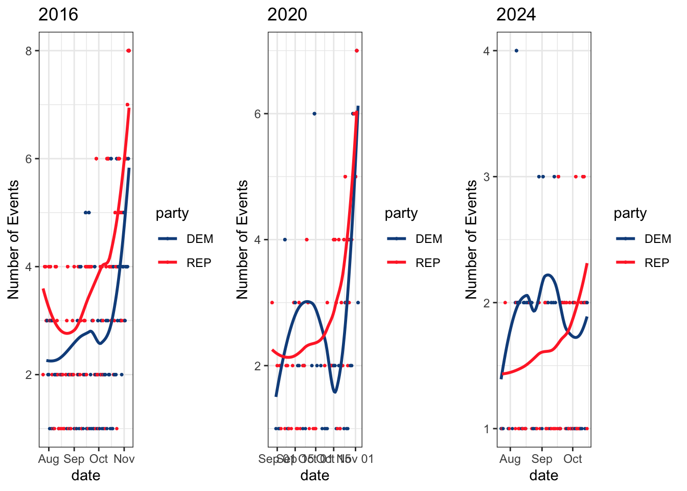
Due to a lack of data surrounding field offices in the 2024 election, I will be using campaign events to measure the effect of the ground game. Campaign events, wherein presidential candidates, their VPs, and their supporters hold rallies, give speeches, or answer questions from the press are one of the most important aspects of the ground game in the days leading up to the election. Indeed, the first figure shows the number of events per day that a campaign will put on in the days leading up to the election. As the first few graphs depict, the number of campaign events per day increases significantly in the immediate lead-up to election day.
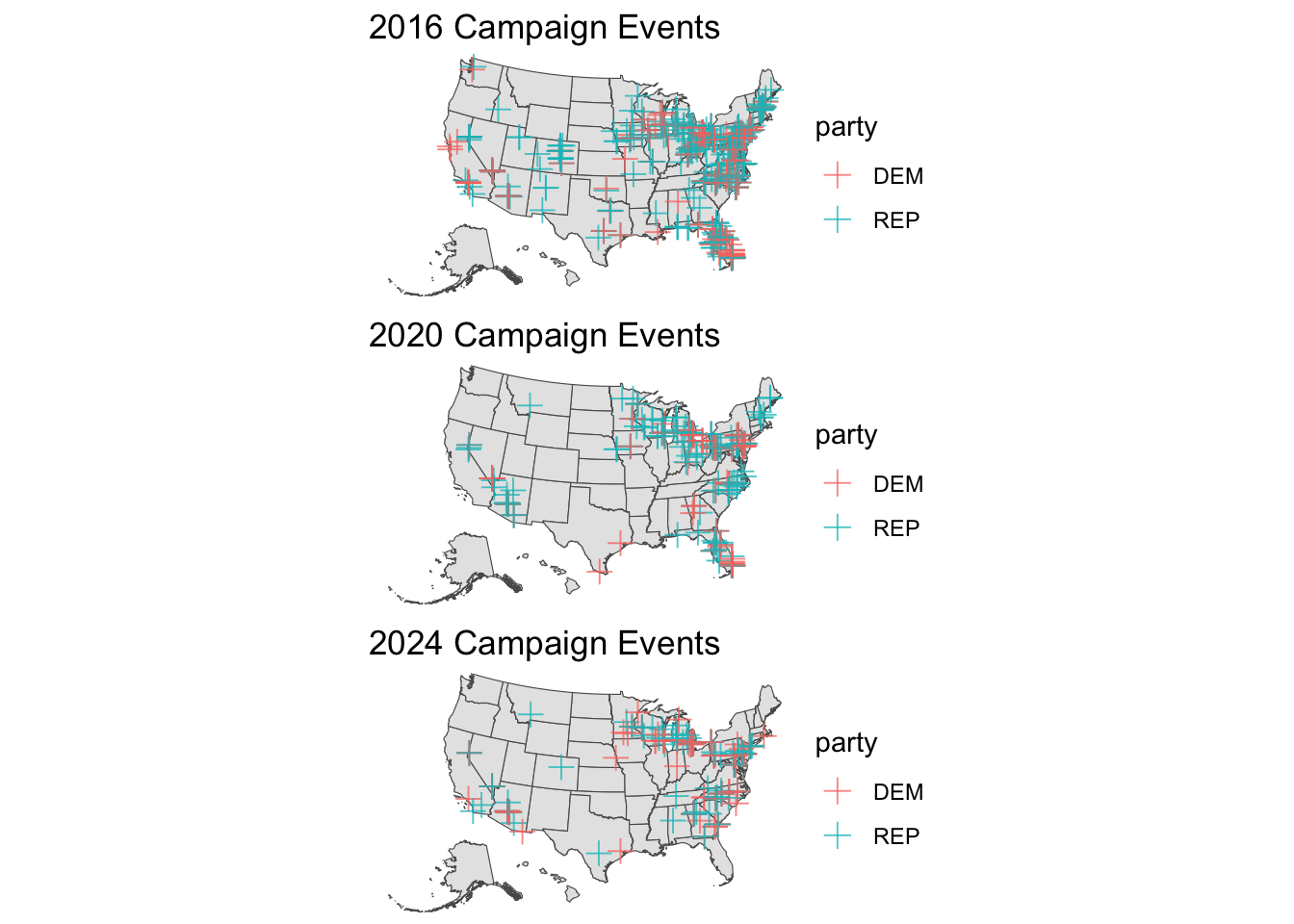
Furthermore, the second group of maps displays the location of these campaign events, indicating that they are often positioned in battle ground states, as the literature discussed above would predict.
##
  |
  |                                                                      |   0%
  |
  |=                                                                     |   1%
  |
  |=                                                                     |   2%
  |
  |===                                                                   |   4%
  |
  |====                                                                  |   5%
  |
  |====                                                                  |   6%
  |
  |=====                                                                 |   7%
  |
  |======                                                                |   8%
  |
  |=======                                                               |  10%
  |
  |========                                                              |  11%
  |
  |=========                                                             |  13%
  |
  |==========                                                            |  14%
  |
  |===========                                                           |  15%
  |
  |===========                                                           |  16%
  |
  |============                                                          |  17%
  |
  |============                                                          |  18%
  |
  |=============                                                         |  19%
  |
  |===============                                                       |  22%
  |
  |================                                                      |  24%
  |
  |==================                                                    |  25%
  |
  |==================                                                    |  26%
  |
  |===================                                                   |  27%
  |
  |====================                                                  |  28%
  |
  |=====================                                                 |  29%
  |
  |=====================                                                 |  30%
  |
  |=====================                                                 |  31%
  |
  |======================                                                |  31%
  |
  |=======================                                               |  33%
  |
  |========================                                              |  34%
  |
  |=========================                                             |  35%
  |
  |==========================                                            |  37%
  |
  |===========================                                           |  39%
  |
  |============================                                          |  40%
  |
  |=============================                                         |  41%
  |
  |==============================                                        |  42%
  |
  |===============================                                       |  44%
  |
  |================================                                      |  46%
  |
  |====================================                                  |  51%
  |
  |=====================================                                 |  52%
  |
  |======================================                                |  54%
  |
  |======================================                                |  55%
  |
  |=======================================                               |  55%
  |
  |========================================                              |  57%
  |
  |==========================================                            |  60%
  |
  |===========================================                           |  61%
  |
  |============================================                          |  63%
  |
  |=============================================                         |  64%
  |
  |==============================================                        |  65%
  |
  |===============================================                       |  67%
  |
  |===============================================                       |  68%
  |
  |=================================================                     |  70%
  |
  |==================================================                    |  71%
  |
  |===================================================                   |  73%
  |
  |====================================================                  |  75%
  |
  |=====================================================                 |  75%
  |
  |=====================================================                 |  76%
  |
  |======================================================                |  77%
  |
  |=======================================================               |  79%
  |
  |========================================================              |  80%
  |
  |========================================================              |  81%
  |
  |=========================================================             |  82%
  |
  |==========================================================            |  83%
  |
  |============================================================          |  85%
  |
  |=============================================================         |  87%
  |
  |=============================================================         |  88%
  |
  |==============================================================        |  89%
  |
  |================================================================      |  91%
  |
  |================================================================      |  92%
  |
  |=================================================================     |  93%
  |
  |===================================================================   |  96%
  |
  |====================================================================  |  97%
  |
  |===================================================================== |  98%
  |
  |======================================================================| 100%
Can the number of campaign events predict state level vote share? The regression below depicts the relationship between the number of Democrat events as well as the difference between the number of events hosted by each party on Democratic two-party vote share. As the regression depicts, these results do not appear to be statistically significant. However, it is also important to run this calculation on a state-by-state basis for the battle ground states so as to understand if this effect can be felt locally.
| Term | Estimate | Std. Error | t value | P-value |
|---|---|---|---|---|
| (Intercept) | 35.5135681 | 1.4807400 | 23.983663 | 0.0000000 |
| n_ev_D | -0.0052570 | 0.0555123 | -0.094700 | 0.9258066 |
| ev_diff_D_R | 0.1175453 | 0.0778413 | 1.510064 | 0.1518031 |
| as.factor(state)Arizona | 14.2259620 | 1.8678033 | 7.616413 | 0.0000016 |
| as.factor(state)California | 30.0689821 | 2.1569598 | 13.940446 | 0.0000000 |
| as.factor(state)Colorado | 18.6013367 | 2.3150191 | 8.035068 | 0.0000008 |
| as.factor(state)Connecticut | 21.6332364 | 2.0904700 | 10.348504 | 0.0000000 |
| as.factor(state)Florida | 13.4233176 | 2.3812276 | 5.637142 | 0.0000473 |
| as.factor(state)Georgia | 13.3435697 | 1.8158822 | 7.348257 | 0.0000024 |
| as.factor(state)Idaho | -3.7061995 | 2.0962391 | -1.768023 | 0.0973853 |
| as.factor(state)Illinois | 23.5169973 | 2.0908608 | 11.247519 | 0.0000000 |
| as.factor(state)Indiana | 5.4504269 | 1.8164412 | 3.000607 | 0.0089616 |
| as.factor(state)Iowa | 10.5893261 | 1.8887167 | 5.606625 | 0.0000500 |
| as.factor(state)Louisiana | 4.2024664 | 2.0890202 | 2.011693 | 0.0625740 |
| as.factor(state)Maine | 17.8577488 | 1.8249599 | 9.785283 | 0.0000001 |
| as.factor(state)Maryland | 28.4997089 | 2.0904700 | 13.633159 | 0.0000000 |
| as.factor(state)Michigan | 15.6545002 | 1.8935746 | 8.267168 | 0.0000006 |
| as.factor(state)Minnesota | 16.9676401 | 1.8238085 | 9.303411 | 0.0000001 |
| as.factor(state)Mississippi | 5.5141298 | 2.0962391 | 2.630487 | 0.0189141 |
| as.factor(state)Missouri | 4.7959302 | 2.0948579 | 2.289382 | 0.0369749 |
| as.factor(state)Montana | 6.2067970 | 2.0962391 | 2.960920 | 0.0097153 |
| as.factor(state)Nebraska | 2.9381140 | 1.8174755 | 1.616591 | 0.1267987 |
| as.factor(state)Nevada | 15.8991896 | 1.8414159 | 8.634220 | 0.0000003 |
| as.factor(state)New Hampshire | 17.1827912 | 1.8878139 | 9.101952 | 0.0000002 |
| as.factor(state)New Jersey | 21.7758790 | 2.0904700 | 10.416738 | 0.0000000 |
| as.factor(state)New Mexico | 19.4898626 | 2.1141959 | 9.218570 | 0.0000001 |
| as.factor(state)New York | 27.5978727 | 2.1596073 | 12.779116 | 0.0000000 |
| as.factor(state)North Carolina | 14.0458813 | 2.0564686 | 6.830098 | 0.0000057 |
| as.factor(state)Ohio | 11.3203157 | 2.0053826 | 5.644966 | 0.0000466 |
| as.factor(state)Oklahoma | -4.8130484 | 2.0904700 | -2.302376 | 0.0360583 |
| as.factor(state)Pennsylvania | 14.9036384 | 2.2521038 | 6.617652 | 0.0000082 |
| as.factor(state)Texas | 10.6153127 | 1.8144597 | 5.850399 | 0.0000319 |
| as.factor(state)Utah | 2.3386241 | 2.1037971 | 1.111621 | 0.2838015 |
| as.factor(state)Virginia | 19.3795812 | 1.9239584 | 10.072765 | 0.0000000 |
| as.factor(state)Washington | 23.2786201 | 2.0904700 | 11.135592 | 0.0000000 |
| as.factor(state)Wisconsin | 15.0050933 | 1.8723613 | 8.013995 | 0.0000008 |
Including campaign events into the 2024 election prediction
As I have done in the previous three weeks, I will be predicting for the seven states which expert predictors like Cook and Sabato determine to be toss-ups in the upcoming election: Arizona, Nevada, Michigan, Wisconsin, North Carolina, Georgia, and Pennsylvania. This prediction model includes the significant variables identified throughout previous analyses including: state vote history as a proxy for demographic and turnout, GDP growth in Q2 before the election, incumbency status, campaign spending, and the latest poll averages. Based off of this week’s analysis, this model will also incorporate campaign events.
| Term | Estimate | Std. Error | t value | P-value |
|---|---|---|---|---|
| (Intercept) | -8.8682324 | 5.8568614 | -1.5141612 | 0.1420479 |
| D_pv2p_lag1 | 0.6003832 | 0.2076646 | 2.8911193 | 0.0076533 |
| D_pv2p_lag2 | -0.1479466 | 0.1619575 | -0.9134899 | 0.3693786 |
| latest_pollav_DEM | 0.5958758 | 0.1401244 | 4.2524771 | 0.0002414 |
| GDP_growth_quarterly | 0.0768032 | 0.0391805 | 1.9602380 | 0.0607666 |
| log(contribution_receipt_amount) | 0.6242280 | 0.4160967 | 1.5001995 | 0.1456093 |
| deminc | NA | NA | NA | NA |
| n_ev_D | -0.0807247 | 0.0339092 | -2.3806136 | 0.0248990 |
| ev_diff_D_R | 0.0897526 | 0.0679365 | 1.3211252 | 0.1979692 |
The table above displays the regression model that has been used to predict the general election outcomes in each battle ground state. According to the regression model, the only statistically significant indicators at the 0.001 level are the latest democratic poll average and the results of the previous election. As has been found repeatedly, Q2 GDP growth is also statistically significant; however, that is only at the 0.1 level. What is interesting is that within this model, the number of Democrat campaign events appears to have a small negative effect on two-party Democratic vote share that is statistically significant at the 0.1 level. This result is most likely biased by limited data within the data set.
Using this model to predict the results in each Battleground state:
| state | prediction | lower_CI | upper_CI | Winner | |
|---|---|---|---|---|---|
| 1 | Arizona | 52.86408 | 48.93663 | 56.79152 | Harris |
| 11 | Nevada | 53.69298 | 49.86749 | 57.51847 | Harris |
| 12 | North Carolina | 52.36521 | 48.43643 | 56.29398 | Harris |
| 13 | Michigan | 54.01648 | 49.98197 | 58.05100 | Harris |
| 14 | Wisconsin | 53.46463 | 49.49467 | 57.43458 | Harris |
| 15 | Georgia | 53.36864 | 49.33574 | 57.40154 | Harris |
| 16 | Pennsylvania | 53.57591 | 49.42734 | 57.72448 | Harris |
As This table displays the results of the model in the seven key battleground states. According to this prediction, Harris will win the election with 319 electoral votes while Trump will have 219 electoral votes.
Notes
All code above is accessible via Github.
Sources
AdImpact. The Play for the White House. October 7, 2024. Accessed October 21, 2024. https://www.wispolitics.com/wp-content/uploads/2024/10/241010AdImpact.pdf.
Enos, Ryan D., and Anthony Fowler. “Aggregate Effects of Large-Scale Campaigns on Voter Turnout.” Political Science Research and Methods 6, no. 4 (2016): 733-51. https://doi.org/10.1017/ psrm.2016.21.
Kalla, Joshua L., and David E. Broockman. “The Minimal Persuasive Effects of Campaign Contact in General Elections: Evidence from 49 Field Experiments.” American Political Science Review 112, no. 1 (2017): 148-66. https://doi.org/10.1017/s0003055417000363.
Data Sources
US Presidential Election Popular Vote Data from 1948-2020 provided by the course. Economic data from the U.S. Bureau of Economic Analysis, also provided by the course. Polling data sourced from FiveThirtyEight and Gallup, also provided by the course. U.S. election spending data from AdImpact as of October 7th.