What role does the campaign play in determining election outcomes?
Throughout the past five weeks, my blog has focused on exploring fundamentals like the economy, polling, incumbency, and demographics. These discussions may generate a false understanding that elections are pre-determined, as they are predictable on a small set of fundamental variables. In reality, fundamentals only represent a partial understanding of the temperature of the American electorate. To truly predict the outcome of presidential elections, it is also important to take into account the 6.6 billion dollar presidential campaign industry.
Presidential campaigns have three main purposes — to convince donors, persuade voters, and mobilize the electorate. There are many mechanisms by which campaigns attempt to fulfill these purposes, the largest of which — the air war of mass media — will be explored below.
What is the air war? How does it influence voters?
To reach the largest number of potential voters, campaigns often turn to mass media to present their message. The meaning of mass media has changed throughout time; however, its largest sector for the past half century has been television advertising. Indeed, according to EMarketer, total US political ad spending will hit $12.32 billion in 2024.
Political advertising has two main effects — persuasion an= mobilization. There are two main pieces of literature which have found proof of the influence of campaign advertising. First, Gerber and his team used a randomized control trial in Rick Perry’s Texas Gubernatorial race to understand the persuasive influence of certain advertisements. By randomizing which county saw what ad, that campaign was able to determine that televised campaign ads have sizable persuasive effects, especially on undecided voters, though those effects tend to fade over time (Gerber et al, 2011). Huber and Arceneaux added to this existing literature with a study of spillover media markets from battleground states, with massive ad funding, into non-battleground states, which typically have almost no ad budget. The authors found that a large influx of advertising, as is often found in battleground states, led places that saw commercials to have their votes changed as compared to the places that did not see the swing-state volume of advertisements (Huber and Arceneaux, 2019).
To understand these effects in practice, is is important to first analyze some descriptive statistics on ads and campaign spending over time.
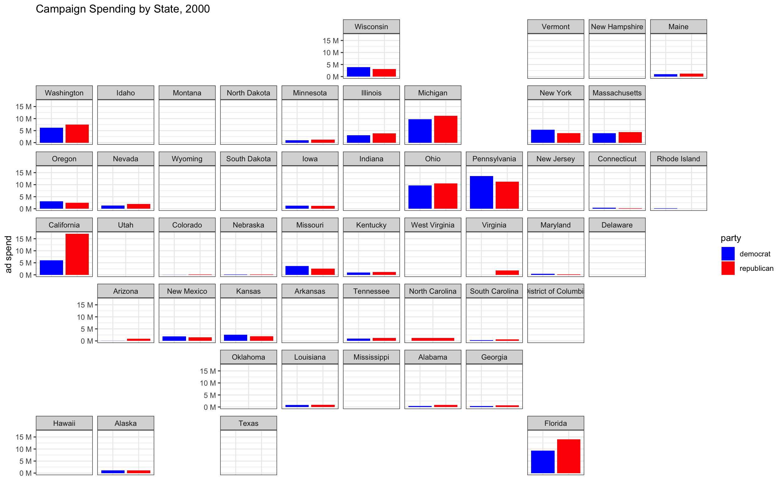
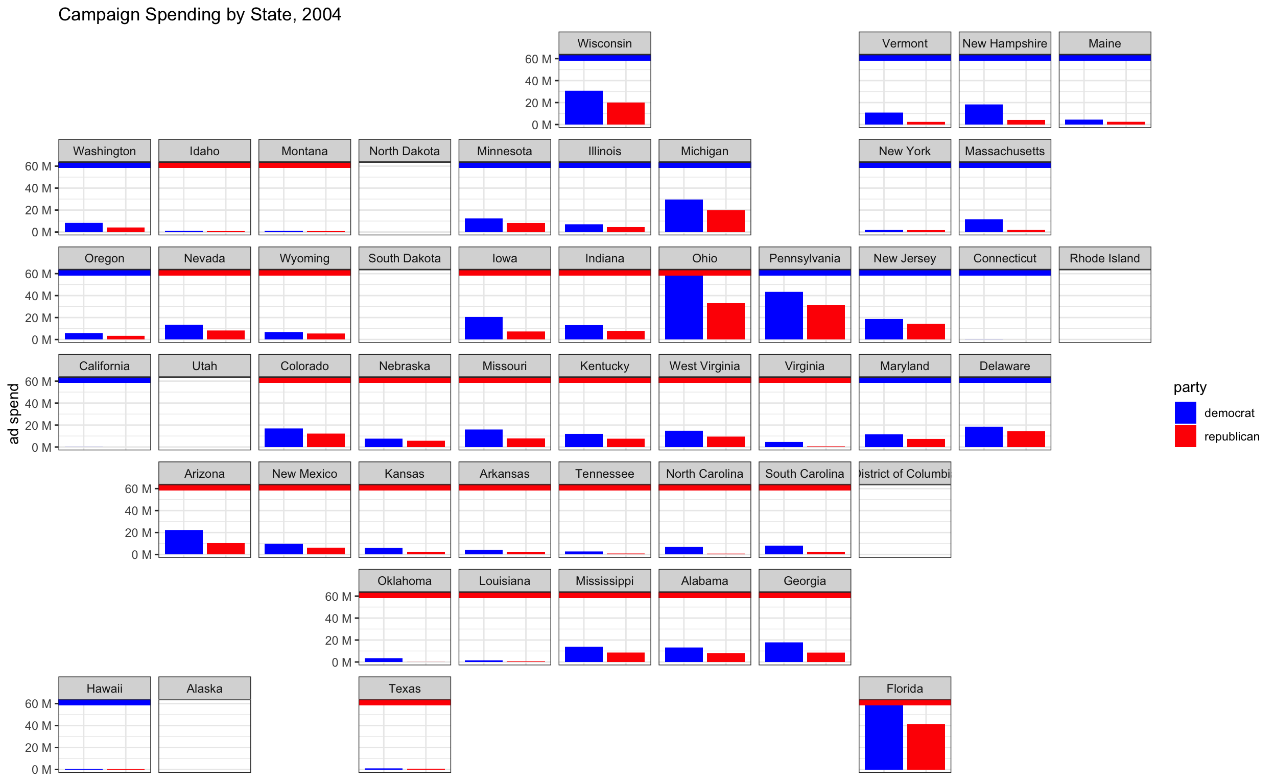
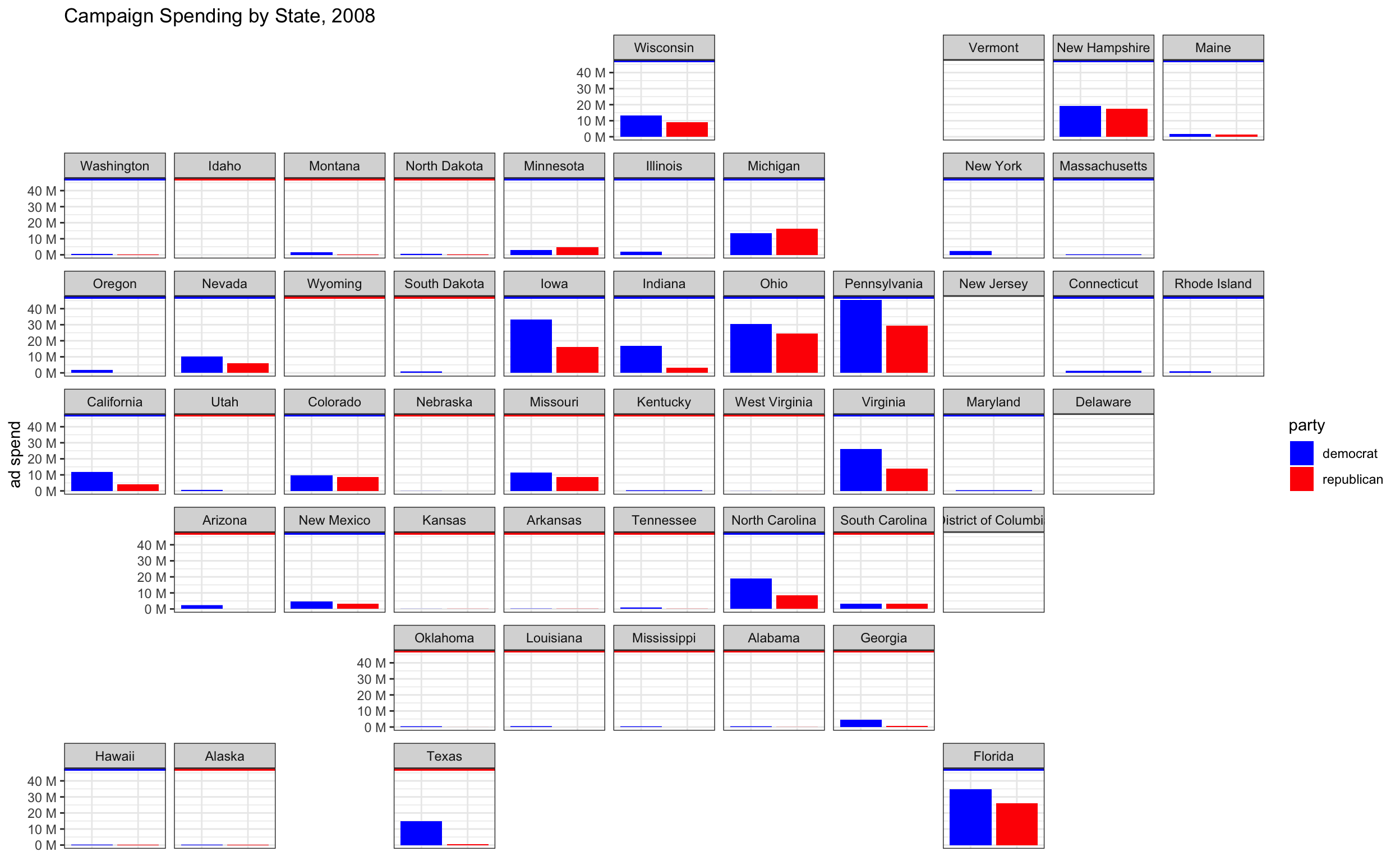
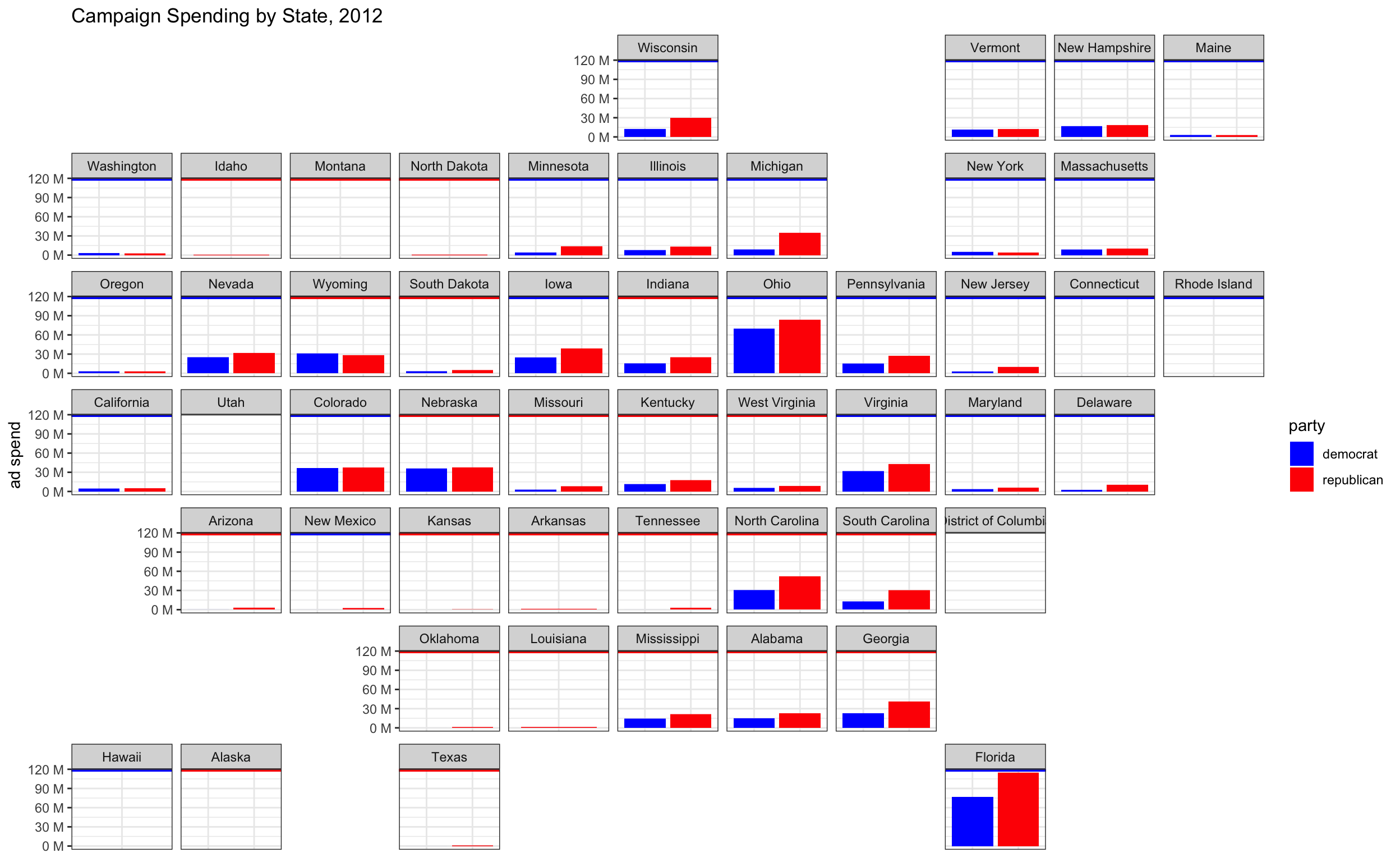
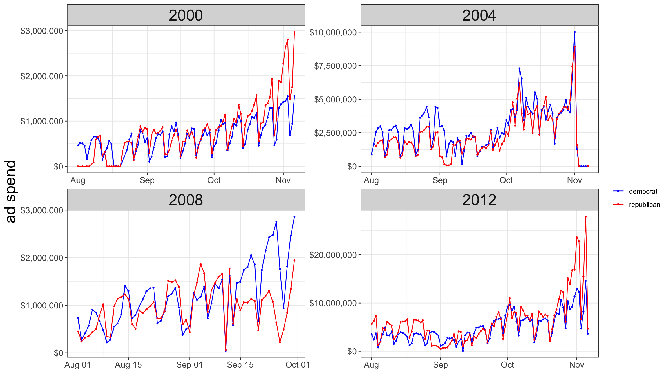
The first four graphics display the volume of campaign spending in the 2000, 2004, 2008, and 2012. These graphics highlight the disparities between election ad spending in swing states vs. non-competitive states. Interestingly, the volume of advertising as well as the states deemed most competitive have changed throughout the years. Generally speaking, however, as elections haev become more competitive over the past 25 years, campaign ad spending has increased dramatically.
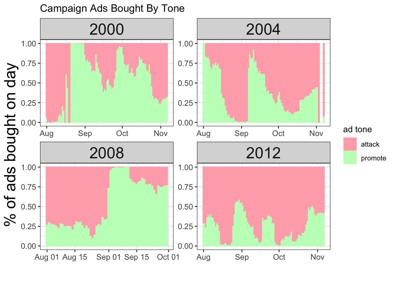
The third emphasizes the timing of this spending, emphasizing the importance of ad spending right before election day due to the lack of ad durability (voters are often unable to retain what they learned in an advertisement for a long period). Both of these graphics also point to an important reality — campaign spending is often evenly matched. Many scholars assert that this equal game of tug-of-war is often why campaigns have a very small effect on outcomes. Indeed, if either party were to let go of the rope, voters may be influenced; however, while the even game continues, neither will make substantial gains.
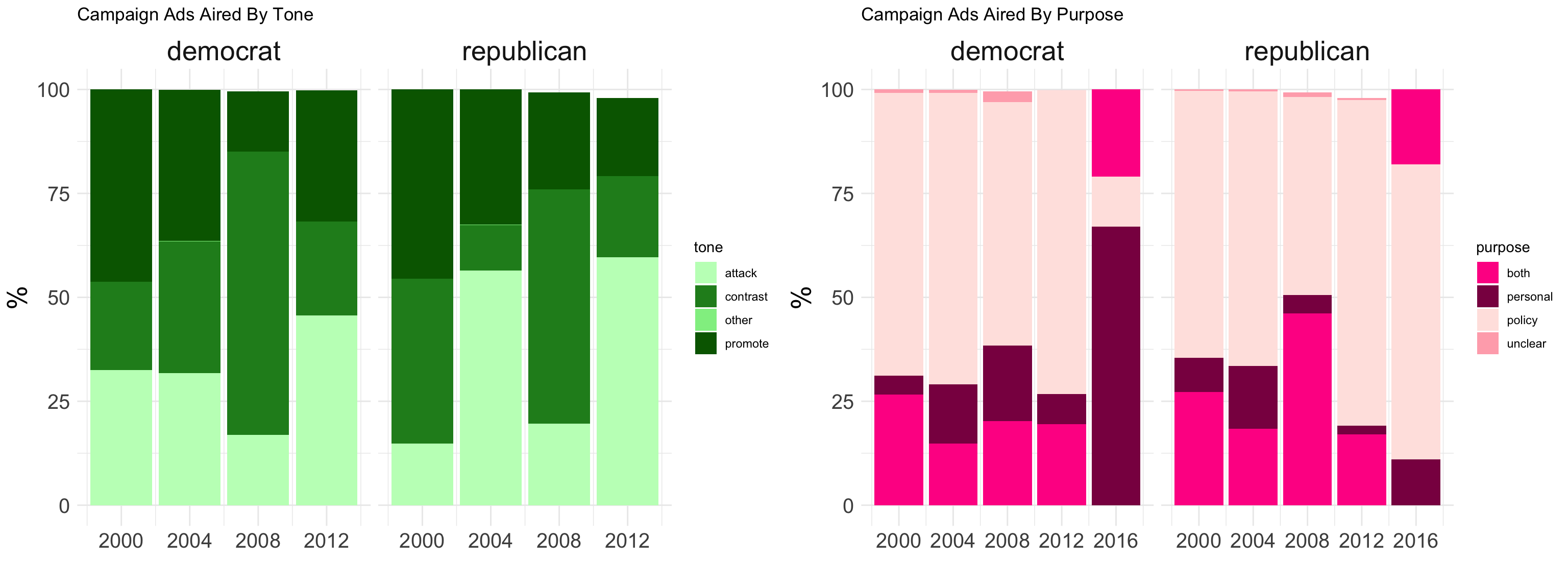
Despite this hypothesis, advertising is still an important way that campaigns convey their message to the general public. Furthermore, despite similarities in the volume of these advertisements, the content differences between parties are immense. The graphics below highlight differentials in terms of the policy and tone of both parties’ advertisements.
The first two explore campaign aids by tone and purpose. For the most part, the proportions in each graph are similar, showing that trends in political advertising content are somewhat consistent. The one exception to this trend would be the purpose of advertisements in 2016. The main reason for this difference is that 2016 data was imputed, as it is not yet available in the correct format.
Furthermore, the figure below emphasizes bipartisan shifts in tone depending on the election cycle. While the 2000 and 2008 campaigns focused on promotional content, 2004 and 2012 carried a lot of attack ads. One potential reason for this could be the role of incumbency, wherein Bush and Obama did not have to focus as heavily on promoting their views while Cheney and Romney were forced to attack the incumbent to make headway in the election.
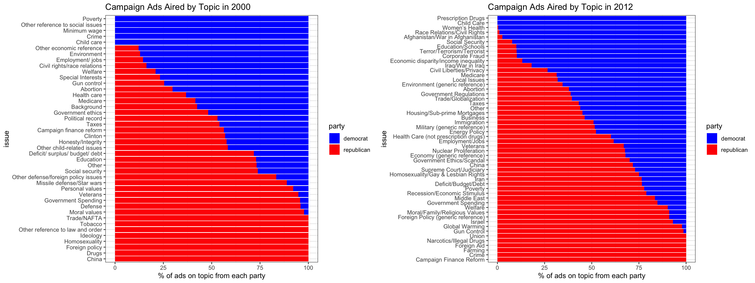
The final figure displays campaign ads aired by issue and party in both 2000 and 2012. As discussed above, there are consistencies across party and year with regard to the tone and purpose of advertising; however, the policy discussed changes substantially depending on the election cycle. As discussed above, advertisements are done with the goal of persuading voters to select a certain candidate. Since fundamental factors cannot be controlled, ads are used to convince voters that a candidate will better serve the electorate on each of these contested factors. As seen by the graphs, in 2000 Democrats were focused on poverty and other social issues while Repulicans were focused on drugs and China. In 2012, however, Republicans were still focused on drugs and crime while democrats were now consumed with the war on Afghanistan.
How can campaign spending be used to predict election outcomes?
To understand the impact of campaign spending on voters, a regression was run which attempted to ascertain this effect. Acknowledging the extreme differences between states in advertising, this relationship was measured at the state level. Furthermore, the values below represent a logistic transformation of this regression so as to normalize the variable which had been right skewed.
Table: Table 1: Estimate State-level Log Regression of Democratic Vote Share on Campaign Spending
| Estimate | Standard Error | z_value | Significance | |
|---|---|---|---|---|
| (Intercept) | 0.8159304 | 12.0532633 | 0.0676937 | |
| log(contribution_receipt_amount) | 2.4419990 | 0.8042939 | 3.0362022 | ** |
| factor(state)Alaska | 4.2876188 | 2.5973042 | 1.6507958 | |
| factor(state)Arizona | 6.4500626 | 2.6698137 | 2.4159223 | * |
| factor(state)Arkansas | -0.5392965 | 2.5335056 | -0.2128657 | |
| factor(state)California | 15.1283965 | 4.0185168 | 3.7646717 | *** |
| factor(state)Colorado | 11.0098622 | 2.8618523 | 3.8471106 | *** |
| factor(state)Connecticut | 17.4150650 | 2.8083447 | 6.2011849 | *** |
| factor(state)Delaware | 21.9221164 | 2.5422100 | 8.6232515 | *** |
| factor(state)Florida | 6.2709580 | 3.1905944 | 1.9654513 | . |
| factor(state)Georgia | 6.4667287 | 2.7703310 | 2.3342802 | * |
| factor(state)Hawaii | 29.4044776 | 2.5296529 | 11.6239178 | *** |
| factor(state)Idaho | -2.8520596 | 2.6009808 | -1.0965323 | |
| factor(state)Illinois | 15.3482805 | 3.1831842 | 4.8216752 | *** |
| factor(state)Indiana | 4.7606831 | 2.5704372 | 1.8520908 | . |
| factor(state)Iowa | 10.7887340 | 2.5313641 | 4.2620238 | *** |
| factor(state)Kansas | 2.8086629 | 2.5350170 | 1.1079464 | |
| factor(state)Kentucky | -0.3147136 | 2.5310771 | -0.1243398 | |
| factor(state)Louisiana | 2.5953805 | 2.5298601 | 1.0258988 | |
| factor(state)Maine | 15.7601823 | 2.5306793 | 6.2276490 | *** |
| factor(state)Maryland | 20.0725361 | 3.0763912 | 6.5247020 | *** |
| factor(state)Massachusetts | 18.4481783 | 3.2127887 | 5.7421076 | *** |
| factor(state)Michigan | 12.0270397 | 2.7598379 | 4.3578791 | *** |
| factor(state)Minnesota | 11.4767922 | 2.7044863 | 4.2436127 | *** |
| factor(state)Mississippi | 7.4131432 | 2.6531495 | 2.7940918 | ** |
| factor(state)Missouri | 4.3124044 | 2.6128251 | 1.6504757 | |
| factor(state)Montana | 6.0957938 | 2.5937352 | 2.3501990 | * |
| factor(state)Nebraska | 2.8530956 | 2.5935430 | 1.1000764 | |
| factor(state)Nevada | 13.6415294 | 2.5407647 | 5.3690643 | *** |
| factor(state)New Hampshire | 13.9049686 | 2.5349624 | 5.4852760 | *** |
| factor(state)New Jersey | 15.3878179 | 2.9666898 | 5.1868646 | *** |
| factor(state)New Mexico | 14.3678855 | 2.5934960 | 5.5399683 | *** |
| factor(state)New York | 14.1120114 | 3.7106795 | 3.8030801 | *** |
| factor(state)North Carolina | 7.5761656 | 2.7965955 | 2.7090673 | ** |
| factor(state)North Dakota | 3.7015153 | 3.0425729 | 1.2165741 | |
| factor(state)Ohio | 7.4366516 | 2.7530734 | 2.7012181 | ** |
| factor(state)Oklahoma | -4.8534329 | 2.5296898 | -1.9185881 | . |
| factor(state)Oregon | 14.2586509 | 2.7295060 | 5.2238943 | *** |
| factor(state)Pennsylvania | 9.1872101 | 3.0027442 | 3.0596047 | ** |
| factor(state)Rhode Island | 23.2334372 | 2.5327104 | 9.1733492 | *** |
| factor(state)South Carolina | 5.6122752 | 2.5386744 | 2.2107109 | * |
| factor(state)South Dakota | 4.9168674 | 2.8422677 | 1.7299100 | . |
| factor(state)Tennessee | -0.5135034 | 2.5962941 | -0.1977832 | |
| factor(state)Texas | 0.6800445 | 3.2117091 | 0.2117391 | |
| factor(state)Utah | -5.7112519 | 2.5307762 | -2.2567194 | * |
| factor(state)Vermont | 26.6027632 | 2.5304299 | 10.5131399 | *** |
| factor(state)Virginia | 9.7776241 | 3.0415112 | 3.2147257 | ** |
| factor(state)Washington | 13.8421205 | 3.0608699 | 4.5222833 | *** |
| factor(state)West Virginia | -1.1641218 | 2.6375444 | -0.4413658 | |
| factor(state)Wisconsin | 12.3481502 | 2.6034893 | 4.7429233 | *** |
| factor(state)Wyoming | -7.1045965 | 2.6995004 | -2.6318190 | ** |
Table: Table 1: Estimate State-level Log Regression of Democratic Two-Party Vote Share on Campaign Spending
| Estimate | Standard Error | z_value | Significance | |
|---|---|---|---|---|
| (Intercept) | 21.4828841 | 10.1575973 | 2.1149573 | * |
| log(contribution_receipt_amount) | 1.0910076 | 0.6777993 | 1.6096321 | |
| factor(state)Alaska | 5.1402035 | 2.1888155 | 2.3483950 | * |
| factor(state)Arizona | 8.5250125 | 2.2499212 | 3.7890272 | *** |
| factor(state)Arkansas | -0.1680661 | 2.1350508 | -0.0787176 | |
| factor(state)California | 21.9097911 | 3.3865083 | 6.4697291 | *** |
| factor(state)Colorado | 14.7628268 | 2.4117571 | 6.1211915 | *** |
| factor(state)Connecticut | 20.0505224 | 2.3666649 | 8.4720581 | *** |
| factor(state)Delaware | 22.1182379 | 2.1423862 | 10.3241132 | *** |
| factor(state)Florida | 9.5976683 | 2.6887966 | 3.5695033 | *** |
| factor(state)Georgia | 8.5343913 | 2.3346297 | 3.6555653 | *** |
| factor(state)Hawaii | 31.6314838 | 2.1318041 | 14.8378945 | *** |
| factor(state)Idaho | -2.7395123 | 2.1919139 | -1.2498266 | |
| factor(state)Illinois | 19.4748350 | 2.6825518 | 7.2598169 | *** |
| factor(state)Indiana | 5.9817390 | 2.1661740 | 2.7614305 | ** |
| factor(state)Iowa | 11.8618955 | 2.1332461 | 5.5604909 | *** |
| factor(state)Kansas | 3.2393226 | 2.1363245 | 1.5163064 | |
| factor(state)Kentucky | 0.0708733 | 2.1330042 | 0.0332270 | |
| factor(state)Louisiana | 2.8431798 | 2.1319787 | 1.3335873 | |
| factor(state)Maine | 17.9890973 | 2.1326690 | 8.4350161 | *** |
| factor(state)Maryland | 24.2955416 | 2.5925546 | 9.3712748 | *** |
| factor(state)Massachusetts | 23.8488694 | 2.7075003 | 8.8084458 | *** |
| factor(state)Michigan | 14.4682817 | 2.3257869 | 6.2208115 | *** |
| factor(state)Minnesota | 14.4609588 | 2.2791406 | 6.3449173 | *** |
| factor(state)Mississippi | 5.9537712 | 2.2358778 | 2.6628339 | ** |
| factor(state)Missouri | 5.8358218 | 2.2018954 | 2.6503628 | ** |
| factor(state)Montana | 6.1978509 | 2.1858078 | 2.8354967 | ** |
| factor(state)Nebraska | 2.6067425 | 2.1856459 | 1.1926646 | |
| factor(state)Nevada | 15.1038182 | 2.1411683 | 7.0540080 | *** |
| factor(state)New Hampshire | 15.0374337 | 2.1362785 | 7.0390792 | *** |
| factor(state)New Jersey | 18.2887892 | 2.5001063 | 7.3152046 | *** |
| factor(state)New Mexico | 17.3546713 | 2.1856063 | 7.9404382 | *** |
| factor(state)New York | 22.8993402 | 3.1270857 | 7.3229013 | *** |
| factor(state)North Carolina | 9.8666775 | 2.3567635 | 4.1865369 | *** |
| factor(state)North Dakota | 1.7548073 | 2.5640550 | 0.6843875 | |
| factor(state)Ohio | 9.7503291 | 2.3200863 | 4.2025717 | *** |
| factor(state)Oklahoma | -4.8382441 | 2.1318352 | -2.2695207 | * |
| factor(state)Oregon | 18.2444226 | 2.3002255 | 7.9315802 | *** |
| factor(state)Pennsylvania | 12.1974354 | 2.5304903 | 4.8201865 | *** |
| factor(state)Rhode Island | 24.2984322 | 2.1343807 | 11.3843009 | *** |
| factor(state)South Carolina | 6.2480604 | 2.1394067 | 2.9204641 | ** |
| factor(state)South Dakota | 3.3758303 | 2.3952526 | 1.4093838 | |
| factor(state)Tennessee | 0.6966264 | 2.1879643 | 0.3183902 | |
| factor(state)Texas | 4.2919034 | 2.7065905 | 1.5857232 | |
| factor(state)Utah | -3.1063815 | 2.1327507 | -1.4565141 | |
| factor(state)Vermont | 29.9205862 | 2.1324588 | 14.0310265 | *** |
| factor(state)Virginia | 13.3402377 | 2.5631603 | 5.2046054 | *** |
| factor(state)Washington | 18.7837061 | 2.5794743 | 7.2819899 | *** |
| factor(state)West Virginia | -2.2158744 | 2.2227270 | -0.9969170 | |
| factor(state)Wisconsin | 14.1205505 | 2.1940279 | 6.4359028 | *** |
| factor(state)Wyoming | -7.8505299 | 2.2749389 | -3.4508750 | *** |
There are many interesting findings within these results:
As contribution amounts increase, the vote percentage difference increases more substantially. This general effect can be seen across both models as well as the varios states within the fixed effect model.
Looking at two-party vote share versus raw vote percentage yields different results. The general coefficient on contribution receipt amount for the regression which analyzes two-party vote share is both larger than that of raw vote percentage as well as statistically significant. This result is surprising as scholars often assume increased spending to have a minimal effect on two-party vote share due to the tug-of-war effect discussed above, wherein both major parties have nearly equal funding.
Looking more closely at the seven swing states in this upcoming election — Arizona, Nevada, Michigan, Wisconsin, North Carolina, Georgia, and Pennsylvania — we see the literature hold that large increases in campaign funding have only marginal effects on two party vote share. For each of the aforementioned states, the coefficients in the second model were substantially lower than those of the first model, indicating that the large influx of spending during the election cycle is often balanced, thus it does not have a major effect on two-party vote share. The data does indicate, however, that the coefficients of each of these states is statistically significant at the 0.001 level.
While campaign spending cannot determine election outcomes, these results indicate that it is a significant part of the story when attempting to predict the outcome of the 2024 election.
Including campaign spending into the 2024 election prediction
As I have done in the previous three weeks, I will be predicting for the seven states which expert predictors like Cook and Sabato determine to be toss-ups in the upcoming election: Arizona, Nevada, Michigan, Wisconsin, North Carolina, Georgia, and Pennsylvania. This prediction model includes the significant variables identified throughout previous analyses including: state vote history as a proxy for demographic and turnout, GDP growth in Q2 before the election, incumbency status, and the latest poll averages. Based off of this week’s analysis, this model will also incoporate campaign ad spending. While past data is provided by the course through AdImpact, the 2024 AdImpact campaign ad data is not yet available. Indeed, the most recent available data is from May when Biden was still the candidate and advertising had not yet picked up. While this data is merely a proxy, it is likely statistically insignificant and may even bias our model (NPR, 2024). To account for this, the data here will be updated as soon as new AdImpacct information becomes available.
| state | prediction | lower_CI | upper_CI | Winner | |
|---|---|---|---|---|---|
| 1 | Arizona | 48.78994 | 45.54016 | 52.03972 | Trump |
| 11 | Nevada | 49.58943 | 46.19746 | 52.98139 | Trump |
| 12 | North Carolina | 48.71165 | 45.37879 | 52.04450 | Trump |
| 13 | Michigan | 50.35126 | 47.08552 | 53.61700 | Harris |
| 14 | Wisconsin | 50.03782 | 46.71100 | 53.36465 | Harris |
| 15 | Georgia | 49.26430 | 46.02230 | 52.50629 | Trump |
| 16 | Pennsylvania | 50.01836 | 46.72100 | 53.31571 | Harris |
This table displays the results of the model in the seven key battleground states. According to this prediction, Harris will win the election with 270 electoral votes while Trump will have 268 electoral votes.
Notes
All code above is accessible via Github.
Sources
Gerber, Alan S., James G. Gimpel, Donald P. Green, and Daron R. Shaw. “How Large and Long-lasting Are the Persuasive Effects of Televised Campaign Ads? Results from a Randomized Field Experiment.” American Political Science Review 105, no. 1 (2011): 135-50. https://doi.org/ 10.1017/s000305541000047x.
Huber, Gregory A., and Kevin Arceneaux. “Identifying the Persuasive Effects of Presidential Advertising.” American Journal of Political Science 51, no. 4 (2007): 957-77. https://doi.org/ 10.1111/j.1540-5907.2007.00291.x.
Montanaro, Domenico. “Ad Spending Shows Where the Presidential Campaign Is Really Taking Place.” NPR. Last modified May 26, 2024. https://www.npr.org/2024/05/24/nx-s1-4980821/ ad-spending-presidential-election-biden-trump.
Data Sources
US Presidential Election Popular Vote Data from 1948-2020 provided by the course. Economic data from the U.S. Bureau of Economic Analysis, also provided by the course. Polling data sourced from FiveThirtyEight and Gallup, also provided by the course. U.S. election soendign data sources from AdImpact.